This article is transferred from: Liu Diwei finishing
Introduction
There are too many machine learning algorithms, classification, regression, clustering, recommendation, image recognition, etc. It is really not easy to find a suitable algorithm. Therefore, in practical applications, we generally use heuristic learning methods to experiment. . Usually we will initially select algorithms that we generally agree with, such as SVM, GBDT, Adaboost. Now that deep learning is very hot, neural networks are also a good choice. If you care about accuracy, the best way is to test the algorithms one by one by cross-validation, compare them, and then adjust the parameters to ensure that each algorithm achieves an optimal solution, and finally choose the best one of. But if you are just looking for a "good enough" algorithm to solve your problem, or some tips here can refer to, to analyze the advantages and disadvantages of each algorithm below, based on the advantages and disadvantages of the algorithm, it is easier for us to choose it.
Deviation & variance
In statistics, whether a model is good or bad is measured in terms of deviations and variances, so we first spread the bias and variance:
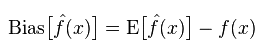
Deviation: Describes the difference between the expected value E' of the predicted value (estimated value) and the actual value Y. The larger the deviation, the more it deviates from the real data.
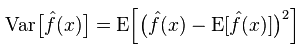
Variance: describes the range of variation of the forecast value P, the degree of dispersion, and the variance of the predicted value, that is, the distance from its expected value E. The larger the variance, the more dispersed the distribution of the data.
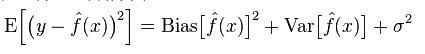
The true error of the model is the sum of the two, as shown below:
In the case of small training sets, high-bias/low-variance classifiers (for example, Naive Bayesian NB) have greater advantages than low-bias/high-variance large categories (for example, KNN) because the latter will overfit. However, as your training set grows, the better the model's ability to predict the original data, the less the bias, and the low-bias/high-variance classifiers will gradually show their advantages (because they have lower gradients Near-error) At this point, the high-deviation classifier is no longer sufficient to provide an accurate model.
Of course, you can also think of this as a difference between the generation model (NB) and the discriminant model (KNN).
Why naive Bayes is a high deviation and low variance?
The following content is quoted from:
First, suppose you know the relationship between the training set and the test set. In simple terms, we need to learn a model on the training set, and then use the test set to use it. The effect is good or bad according to the error rate of the test set. But many times, we can only assume that the test set and training set are in line with the same data distribution, but they can't get real test data. At this time, how can you measure the error rate when you only see the training error rate?
Because the training sample is very few (at least not enough), the model obtained through the training set is not always true. (Even if the correct rate is 100% on the training set, it does not mean that it portrays the real data distribution. It is our purpose to describe the actual data distribution, not just the limited data points of the training set). Moreover, in practice, training samples often have a certain noise error, so if you pursue the perfection of the training set and adopt a very complicated model, the model will make the errors in the training set be real data distribution characteristics. And thus get an erroneous data distribution estimate. In this case, the real test set is wrong (this phenomenon is called overfitting). However, we cannot use too simple models. Otherwise, when the data distribution is more complex, the model is insufficient to describe the data distribution (embodied as the error rate of the training set is high, this phenomenon is less than the fitting). Overfitting indicates that the model used is more complex than the actual data distribution, while underfitting means that the model used is simpler than the actual data distribution.
In the framework of statistical learning, when people describe the complexity of the model, there is such a view that Error = Bias + Variance. Here, the Error can be roughly understood as the prediction error rate of the model, which is composed of two parts. One is the inaccurate part (Bias) caused by the model being too simple, and the other is due to the complexity of the model. Greater room for change and uncertainty.
Therefore, it is easy to analyze naive Bayes. It simply assumes that the data is irrelevant and is a model that has been greatly simplified. Therefore, for such a simple model, the Bias part is greater than the Variance part in most occasions, that is to say high deviation and low variance.
In practice, in order to make Error as small as possible, we need to balance the proportion of Bias and Variance when choosing models, that is, balance over-fitting and under-fitting.
The relationship between deviation and variance and model complexity is more clear using the following diagram:
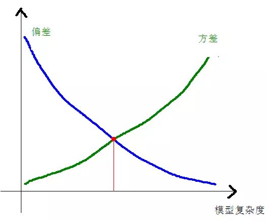
When the complexity of the model rises, the deviation will gradually decrease, and the variance will gradually increase.
Advantages and disadvantages of common algorithms
1. Naive Bayes
Naive Bayes belongs to a generative model (for generation models and discriminative models, mainly whether or not a joint distribution is required). It is very simple. You just do a bunch of counting. If you note conditional independence (a more stringent condition), the naive Bayesian classifier will converge faster than a discriminative model, such as logistic regression, so you only need less training data. Even though the NB conditional independence assumption does not hold, the NB classifier still performs very well in practice. Its main drawback is that it cannot learn the interactions between features. In RRM in mRMR, it is feature redundancy. Citing a more classic example, for example, although you like the movie Brad Pitt and Tom Cruise, it can't learn that you don't like the movie they are playing together.
advantage:
Naive Bayesian model originated from the classical mathematical theory, has a solid mathematical foundation, and stable classification efficiency.
Good performance on small-scale data, able to deal with multi-category tasks, suitable for incremental training;
Not very sensitive to missing data, the algorithm is also relatively simple and is often used for text classification.
Disadvantages:
Need to calculate the prior probability;
Classification decision has an error rate;
Very sensitive to the form of input data.
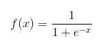
2. Logistic Regression
Belonging to discriminative models, there are many methods for regularizing models (L0, L1, L2, etc), and you don't have to worry about whether your features are relevant, as you would with naive Bayes. Compared with the decision tree and the SVM, you will also get a good explanation of the probability that you can even use the new data to update the model (using online gradient descent). If you need a probabilistic framework (eg, simply adjust classification thresholds, indicate uncertainty, or get confidence intervals), or if you want to quickly integrate more training data into the model later, use it.
Sigmoid function :
Advantages :
Simple implementation, widely used in industrial issues;
When the classification is very small, the calculation speed is very fast, and the storage resources are low;
Convenient observation sample probability score;
For logistic regression, multicollinearity is not a problem. It can be combined with L2 regularization to solve this problem.
Disadvantages :
When the feature space is large, the performance of logistic regression is not very good;
Easy to under-fit, the general accuracy is not too high
Not deal with a large number of features or variables;
Can only deal with two classification problems (softmax derived from it can be used for multiple classification), and must be linearly separable;
For non-linear features, conversion is needed;
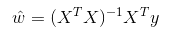
3. Linear regression
Linear regression is used for regression. Unlike Logistic regression, it is used for classification. The basic idea is to use the gradient descent method to optimize the error function in the form of least squares method. Of course, the solution to the parameters can also be obtained directly using the normal equation. The result is:
In LWLR (Local Weighted Linear Regression), the expression for the parameter is:
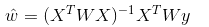
This shows that LWLR is different from LR, and LWLR is a non-parametric model because each time the regression calculation is performed, it must traverse the training sample at least once.
Advantages : Simple to implement, simple to calculate;
Disadvantages : Cannot fit non-linear data.
4. Recently led the algorithm - KNN
KNN is the nearest neighbor algorithm and its main process is:
1. Calculate the distance between each sample point in the training sample and the test sample (common distance measures are Euclidean distance, Mahalanobis distance, etc.); 2. Sort all distance values ​​above; 3. Select the k minimum distances before Samples; 4. Voting based on the labels of the k samples to get the final classification category;
How to choose an optimal K value depends on the data. In general, larger K values ​​can reduce the effect of noise during classification. But it will blur the boundaries between categories. A good K value can be obtained through various heuristic techniques, such as cross-validation. In addition, the presence of noise and non-correlation feature vectors will reduce the accuracy of the K nearest neighbor algorithm.
The nearest neighbor algorithm has a strong consistency result. As the data tends to be infinite, the algorithm guarantees that the error rate will not exceed twice the Bayesian algorithm error rate. For some good K values, K nearest neighbors guarantee that the error rate will not exceed the Bayesian theoretical error rate.
The advantages of KNN algorithm
The theory is mature and the idea is simple. It can be used both for classification and regression.
Can be used for nonlinear classification;
The training time complexity is O(n);
There are no assumptions about the data, high accuracy, and insensitivity to outliers;
Shortcomings
Large amount of calculation;
Sample imbalance problem (that is, there are a large number of samples in some categories, and a small number of other samples);
Need a lot of memory;
5. Decision tree
Easy to explain. It can handle interactions between features without stress and is non-parametric, so you don't have to worry about outliers or whether the data is linearly separable (for example, a decision tree can easily handle category A in a feature dimension x At the end, the category B is in the middle, and then the category A reappears in the front of the feature dimension x). One of its shortcomings is that it does not support online learning. Therefore, after the arrival of a new sample, the decision tree needs to be completely rebuilt. Another disadvantage is that it is prone to overfitting, but it is also the point of entry for integration methods such as Random Forest RF (or boosted tree). In addition, Random Forest is often the winner of many classification problems (usually better than the SVM). It is fast and adjustable, and you don't have to worry about adjusting a lot of parameters like a support vector machine. So before It has always been very popular.
An important point in the decision tree is to choose an attribute for branching, so pay attention to the formula for calculating the information gain and understand it in depth.
Information entropy is calculated as follows:
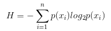
Where n represents n classification categories (eg, the hypothesis is a type 2 problem, then n=2). Calculate the probabilities p1 and p2 of these two types of samples in the total sample, and then calculate the information entropy before the unselected attributes branch.
Now select an attribute xixi for branching. The branching rule is: if xi=vxi=v, the sample is divided into one branch of the tree; if it is not equal, another branch is entered. Obviously, the sample in the branch is likely to include two categories. Calculate the entropy H1 and H2 of the two branches and calculate the total information entropy H' = p1H1+p2 H2. Then the information gain ΔH = H - H'. Based on the information gain principle, all attributes are tested on one side, and one attribute that maximizes gain is selected as the current branch attribute.
The advantages of the decision tree itself:
Simple calculation, easy to understand, strong interpretability;
More suitable for processing samples with missing attributes;
Ability to deal with irrelevant features;
In a relatively short period of time, it is possible to make feasible and effective results for large data sources.
Shortcomings
Overfitting is easy to happen (random forests can reduce overfitting to a great extent);
Ignoring the correlation between data;
For data with inconsistent sample sizes for each category, the information gains in the decision tree are biased towards those features that have more numerical values ​​(as long as the information gains are used, there are drawbacks such as RF).
5.1 Adaboosting
Adaboost is a summation model. Each model is based on the error rate of the previous model. It pays too much attention to the wrong samples, and reduces the degree of attention to the correctly classified samples. After successive iterations, it can be compared. Good model. Is a typical boosting algorithm. The following is a summary of its advantages and disadvantages.
advantage
Adaboost is a very precise classifier.
Various methods can be used to build sub-classifiers. The Adaboost algorithm provides a framework.
When using a simple classifier, the calculated results are understandable, and the construction of the weak classifier is extremely simple.
Simple, no feature screening.
Overfitting is not easy to happen.
For combinatorial algorithms such as Random Forest and GBDT, refer to this article: Machine Learning - Combination Algorithms Summary
Disadvantages : sensitive to outliers
6.SVM support vector machine
The high accuracy provides a good theoretical guarantee for avoiding over-fitting, and even if the data is linearly indivisible in the original feature space, it will work well if given a suitable kernel function. It is especially popular in the high-dimensional text classification problem. Unfortunately, memory is expensive, difficult to explain, running and adjusting parameters are also annoying, and Random Forest just avoid these shortcomings, more practical.
advantage
Can solve high-dimensional problems, that is large-scale feature space;
Ability to handle interactions of non-linear features;
No need to rely on the entire data;
Can improve the generalization ability;
Shortcomings
When there are many observations, the efficiency is not very high;
There is no universal solution to nonlinear problems. Sometimes it is difficult to find a suitable kernel function.
Sensitive to missing data;
The selection of the kernel is also tricky (libsvm comes with four kernel functions: linear kernel, polynomial kernel, RBF, and sigmoid kernel):
First, if the number of samples is smaller than the number of features, then there is no need to choose nonlinear kernels. Simply use linear kernels.
Second, if the number of samples is greater than the number of features, nonlinear kernels can be used at this time, and mapping the samples to higher dimensions generally yields better results.
Third, if the number of samples and the number of features are equal, a non-linear kernel can be used in this case, and the principle is the same as the second one.
For the first case, you can also reduce the dimension of the data first, and then use a nonlinear kernel, which is also a method.
7. The advantages and disadvantages of artificial neural networks
The advantages of artificial neural networks :
The accuracy of the classification is high;
Parallel distribution processing capability, strong ability to distribute storage and learning,
It has strong robustness and fault-tolerance ability to noise nerves, and can fully approximate complex nonlinear relationships.
With associative memory function.
Disadvantages of artificial neural networks :
Neural networks require a large number of parameters, such as the initial value of the network topology, weights and thresholds;
Can not observe the learning process between, the output is difficult to explain, will affect the credibility and acceptability of the results;
If you study too long, you may not even reach the goal of learning.
8, K-Means clustering
Previously written an article on K-Means clustering, blog post link: machine learning algorithm-K-means clustering. About the derivation of K-Means, there is a very strong EM thinking.
advantage
The algorithm is simple and easy to implement;
For processing large data sets, the algorithm is relatively scalable and efficient because its complexity is approximately O(nkt), where n is the number of all objects, k is the number of clusters, and t is the number of iterations. Usually k< The algorithm attempts to find the k divisions that minimize the squared error function value. When the clusters are dense, spherical or agglomerated, and the clusters differ significantly from each other, the clustering effect is better. Shortcomings High data type requirements, suitable for numerical data; May converge to a local minimum and converge slowly on large-scale data K value is more difficult to choose; Sensitivity to the initial value of the cluster center, for different initial values, may lead to different clustering results; It is not suitable for finding clusters with non-convex shapes or clusters with large differences in size. Sensitive to "noise" and outlier data, a small amount of this data can have a large impact on the average value. Algorithm Selection Reference Prior to translation of some foreign articles, there is a simple algorithm selection technique given in an article: 1. The first choice should be to choose the logistic regression. If its effect is not good, then its results can be used as a reference, and compared with other algorithms on the basis; 2. Then try the decision tree (random forest) to see if you can significantly improve your model's performance. Even if you don't use it as a final model at the end, you can use random forests to remove noise variables for feature selection. 3. If the number of features and observations are particularly large, then when resources and time are sufficient (this premise is important), using SVMs is an option. Normally: GBDT>=SVM>=RF>=Adaboost>=Other... Now that deep learning is very popular, it is used in many fields. It is based on neural networks and I am currently learning it myself, only theoretical knowledge Not very solid, not deep enough to understand, not to introduce here. Although the algorithm is important, good data is better than good ones , and designing good features is of great benefit. If you have a very large data set, then no matter which algorithm you use may have little effect on the classification performance (at this point you can make choices based on speed and ease of use). This article has been transferred from Big Data Talent Network. If you need to reprint, please contact the original author. Electroplating Rectifier Equipment Plating Power Supply,Chrome Plating Power Supply,Copper Plated Ower Supply,Zinc-Ni Crs Power Supply Shaoxing Chengtian Electronic Co., Ltd. , https://www.ctnelectronicpower.com