Filter Basics: Anti-aliasing

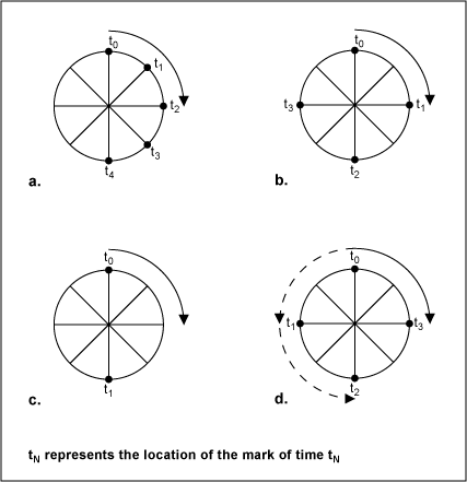
Filtering is a common process that we often take for granted. When we are on the phone, the receiver filters out all other channels so that we only receive the specific channel. When we adjust the equalizer of the stereo system, the bandpass filter is used to selectively increase or decrease the audio signal of a specific frequency band.

Filters play an important role in almost all data sampling systems. Most analog-to-digital converters (ADCs) are equipped with filters that filter out frequency components outside the ADC range. Some ADCs have filtering on their structure itself.

We next discuss the data sampling system, filtering requirements, and the relationship to aliasing.

The maximum frequency component that the data sampling system can process with high precision is called its Nyquist limit. The sample rate must be greater than or equal to twice the maximum frequency of the input signal. If this rule is violated, unwanted or harmful signals appear in the useful frequency band, called "aliasing."

For example, to digitize a 1 kHz signal, a minimum sample rate of 2 kHz is required. In practical applications, the sampling rate is usually higher to provide a certain margin and reduce the filtering requirements.

To help understand data sampling systems and aliasing, we take traditional film photography as an example.

In the old West, when the carriage accelerates, the wheels accelerate normally, and then it seems that the wheel speed is slower, and then it seems to stop. When the carriage is further accelerated, the wheels look like they are turning backwards. In fact, we know that the carriage did not go backwards because everything else was normal. What caused this phenomenon? The answer is: the frame rate is not high enough to accurately capture the rotation of the wheel.

To help understand, assume that a visible mark is placed on the wagon wheel and the wheel turns. Then we take photos (or samples) by time. Since a movie camera captures motion by capturing a certain number of photos per second, it is essentially a data sampling system. Just as film uses discrete images of the wheel, the ADC captures a series of snapshots of the motion electrical signal.

When the carriage is first accelerated, the sampling rate (the frame rate of the movie camera) is much higher than the rotation speed of the wheel, so the Nyquist condition is satisfied. The camera's sampling rate is higher than twice the wheel speed, so we can accurately describe the movement of the wheel. We see how the wheel accelerates (Figures 1a and 1b).

At the Nyquist limit, we see two points in the 180 degree range (Fig. 1c). It is generally difficult for the human eye to clearly distinguish the time between these two points. These two points appear at the same time, and the wheels appear to stop. At this wheel speed, the rate of rotation is known (according to the sampling rate), but the direction of rotation is not known. When the carriage continues to accelerate, the Nyquist condition is no longer satisfied, and there are two possible ways to see the wheel: we “see” the wheel in the forward direction, while others see it is reversed (Fig. 1d).

Figure 1. An example of a wagon wheel.

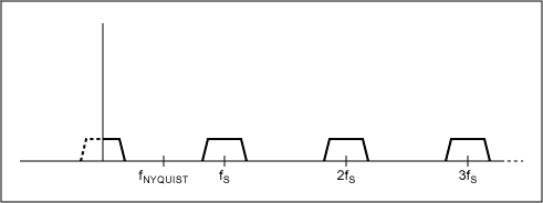
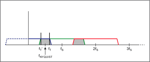
Both directions can be seen as the right direction, depending on how you “see” the wheel, but we know that signal aliasing has occurred. That is to say, harmful frequency components appear in the system, we can't distinguish it from the real value, and there are motion information of forward and reverse. We generally see the "about" or "mirror" of the inverted component or the forward component. Since the data is processed in a combination of eye/brain, we are not aware of the main information about wheel forwarding. Another interesting phenomenon is that when the sampling rate is exactly equal to the wheel speed, the data provides little useful information because the mark always appears at the same position on the wheel. In this case, no one can know if the wheel is spinning or still.

Now move to the field of mathematics, assuming the wheel is a unit circle, using sine and cosine coordinates. If the forward and negative peaks of the cosine value are sampled (180 degrees out of phase), then the Nyquist condition is satisfied and the original cosine value can be reconstructed using the two sampled data points. Therefore, the Nyquist limit is the key to reconstructing the original signal. As more points are added, the ability to reproduce the original signal increases.

Going to the frequency domain, Figure 2 shows the frequency response of the sampled data system. Note that the data is repeated at multiples of the sample rate ("mirror" of the original signal); this is a fundamental feature of the sampled data system. In Figure 2a, the Nyquist condition is satisfied and there is no aliasing in the useful band. However, in Figure 2b, since the highest frequency in the useful band is greater than one-half the sampling rate, the Nyquist condition is no longer satisfied. The overlapping regions are aliased; the signal with the frequency fT also appears at fT', similar to the aliasing of the wagon wheels.

Figure 2a. Sampling data system frequency response, no aliasing.

Figure 2b. Sampling data system frequency response with aliasing.

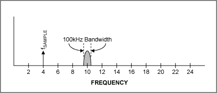
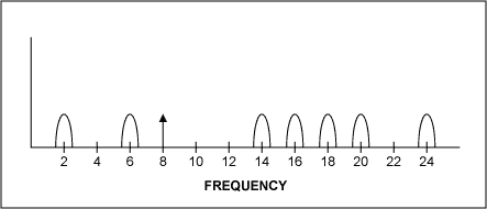
Undersampling is a powerful tool that can be used effectively in selected applications. Undersampling allows the ADC to act as a mixer that can receive modulated high frequency carrier signals and produce lower frequency mirrors. In this way, it is like a downconverter. Another major advantage is that the ADC's sampling rate is lower than the Nyquist frequency, which generally has a significant cost advantage. For example, suppose the modulation carrier is 10 MHz, the bandwidth is 100 kHz (±50 kHz, and the center frequency is 10 MHz). Undersampling at 4MHz yields 1st order sum and difference terms (f1 + f2 and f1 - f2), 14MHz and 6Mz, respectively; 2nd order terms (2f1, 2f2, 2f1 + f2, f1 + 2f2, | 2f1 - f2 | , | f1 - 2f2 |), 8MHz, 20MHz, 18MHz, 2MHz, 24MHz and 16MHz. The image signal appearing at 2 MHz is a useful signal. Note that our original signal is at 10MHz and is mirrored at 2MHz by digitizing it. Now we can perform signal processing (filtering and mixing) in the digital domain to recover the original 50kHz signal. This process does not require significant simulation processing, which is one of its main advantages. Since all processing is done in the digital domain, you only need to modify the software if you need to make changes to the performance and features of the circuit. In contrast, for analog designs, if you need to change the circuit performance, you need to change the hardware components and layout of the circuit, and the cost is quite high.

One disadvantage of undersampling is that harmful signals can occur in the useful frequency band and you cannot distinguish it from useful signals. In addition, the frequency range of the ADC input is often very wide when undersampling. In the above example, even if the sample rate is 4MHz, the ADC front end must still sample the 10MHz signal. In contrast, if the analog carrier is moved down the baseband to the baseband before the ADC, the input bandwidth of the ADC needs to be only 50kHz instead of 4MHz, reducing the ADC front-end and input filtering requirements.

Figure 3a. Example of undersampling.

Figure 3b. Undersampled digitized image signal (1st order and 2nd order).

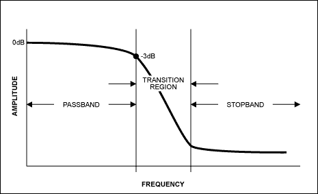
Oversampling provides a so-called processing gain. In oversampling, the actual required number of samples is obtained at a higher sampling frequency, and then the data is filtered, thereby effectively reducing the noise floor of the system (assuming the noise is broadband white noise). This is different from averaging, the latter is to get a lot of samples and the noise is averaged. Oversampling can be understood as follows: If the input signal comes from a source of scanning frequency, the spectrum can be divided into multiple ranges or "containers" with a fixed bandwidth per container. Broadband noise is spread over the entire useful frequency range, so each container has a certain amount of noise. Now, if the sampling rate is increased, the number of frequency containers is also increased. In this case, the amount of noise that appears is still the same, but we have more containers to accommodate the noise. Then we use filters to filter out noise that is outside the useful band. The result is a reduction in noise per container, so the over-sampling effectively reduces the noise floor of the system.

For example, if we have a 2ksps ADC (using the 1kHz Nyquist limit in the following equation) and a 1kHz signal, the ADC is followed by a 1kHz digital filter, and the processing gain is given by: -10 &TImes; log (1kHz/1kHz ) = 0dB. If we increase the sample rate to 10ksps, the processing gain is now -10 &TImes; log (1kHz/5kHz) = 7dB, or about 1 bit resolution (1 bit is roughly equivalent to a 6dB improvement in signal-to-noise ratio (SNR)). With oversampling, the noise is not reduced, but is spread over a wider bandwidth; placing some of the noise outside of the useful bandwidth is equivalent to reducing noise. This noise improvement is based on the following formula:

SNR improvement (dB) = 10 &TImes; LOGA/B, where A is equal to noise and B is equal to oversampling noise.

Another way to express this process is that oversampling reduces the in-band RMS quantization noise and the coefficient is the square root of the oversampling rate. Or, if the noise is reduced by a factor of two, it is equivalent to a 3dB effective processing gain. Don't forget, we only discussed broadband noise here. Oversampling cannot simply eliminate other noise sources and other errors.

With the above background, we now discuss anti-aliasing filters. When selecting a filter, the goal is to provide a cutoff frequency that eliminates unwanted signals from the ADC input or at least attenuates it without negatively affecting the circuit. Anti-aliasing filters are low pass filters that meet this requirement. How to choose the right filter? The key parameters to consider are the amount of attenuation (or ripple) in the passband, the expected filter roll-off within the stopband, the steepness of the transition region, and the phase relationship of the different frequencies through the filter (Figure 4a).

Figure 4a. Actual filter.

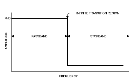
The ideal filter has a "brick wall" response (Fig. 4b), which means that its transition ratio is infinite. However, this is not possible in practical applications. The steeper the roll-off, the higher the "Q" or quality factor of the filter; the higher the Q factor, the more complex the filter design. A higher Q factor can cause the filter to be unstable and self-oscillate at the corresponding corner frequency. The key to choosing a filter is to understand the frequency of the interfering signal and the corresponding amplitude. For example, for a cell phone, the designer knows the worst-case operating condition magnitude and position of the adjacent signal to design it in a targeted manner. Not all signals can be predicted in the frequency domain, and even some known interference signals are too large to be sufficiently attenuated. However, depending on the environment and application, you can consider known interference and design to minimize random interference and ensure more reliable work.

Figure 4b. Ideal filter.

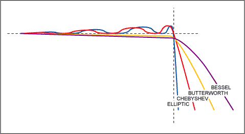
Once the useful signal frequencies are known, a simple filter is used to determine the desired filter structure to meet the passband, stopband, and transition region requirements. Each of the four basic filter types has its own advantages (Figure 5).

Figure 5. Four basic filter types

For example, the Butterworth filter has the flattest passband region, which means that the attenuation is minimal in the corresponding frequency range; the Bessel filter has a flat rolloff, but its main advantage is the linear phase response. That means that the delay of each frequency component as it passes through the filter is equal; since the group delay is defined as the deviation of the phase response from the frequency, the linear phase response is usually referred to as the fixed group delay. The Chebyshev filter has a steeper roll-off, but has a larger ripple in the passband. The elliptical (EllipTIc) filter has the steepest roll-off. For the simplest anti-aliasing filters, simple single-pole passive RC filters are often acceptable. In other cases, active filters (ie, using op amps) are suitable. One advantage of active filters is the multi-order filter, which is less sensitive to external component values, especially the "Q" value of the filter.

The anti-aliasing filter usually does not have to strictly correspond to the position of the inflection point frequency, so there is a certain margin in design. For example, if you need maximum flatness but still have too much attenuation in the passband, just move the corner frequency farther to solve the problem. If the stopband attenuation is too small, the number of poles of the filter can be increased. Another solution is to amplify the signal after filtering to increase the amplitude of the signal relative to the unwanted signal.

Maxim offers a wide range of low-power, low-pass filters for anti-aliasing; including the MAX7490 general-purpose switched-capacitor filter, the MAX740x/MAX741x family's smallest low-power, low-pass switched-capacitor filters, and the MAX274 /MAX275 Universal Continuous Time Mode Filter. Maxim also offers a wide range of low-power, high-precision op amps for users who want to design their own filters. For these users, it is highly recommended to refer to the good filter manual during the design process.